

Week 3: Sequence models & Attention mechanism

In this series, we will look primarily at sequence models, which are useful for everything from machine translation to speech recognition. We will also look at attention models.

Sequence models & Attention mechanism: Basic Models

Machine translation

Lets say we want to translate from french to english. We will use the following examples:

$$x: \text{"Jane visite l'Afrique en septembre"}$$

$$y: \text{"Jane is visiting Africa in September"}$$

Recall that we represent individual elements in the input sequence as $x^{<t>}$, and in the output sequence as $y^{<t>}$.

Most of the ideas presented in this lecture are from this paper and this paper.

First, we build our encoder, an RNN (LSTM or GRU) which processes the input sequence. The encoder outputs a vector that represents the learned representation of the input sequence. A decoder takes this output sequence, and outputs the translation one word at a time.

Note that the outputs from each timestep in the decoder network are actually passed as input for the next timestep in the case of language modelling.

Given enough data, this sequence to sequence architecture actually works quite well.

Image captioning

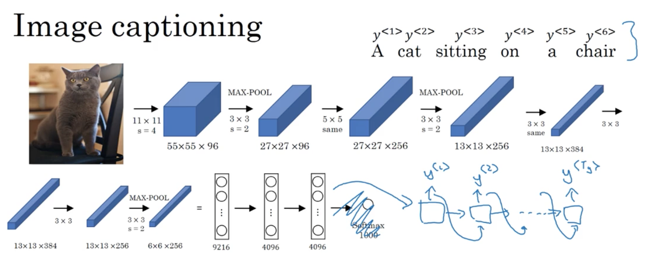
The task of image captioning involves inputing an image, and having the network generate a natural language caption.

$$x: \text{an image of a cat of a chair}$$

$$y: \text{"A cat sitting on a chair"}$$

Typically, we use a CNN as our encoder, without any classification layer at the end. We feed the learned representation to a decoder, an RNN, which generates and output sequence which is our image caption.

Summary

• Simple sequence to sequence (seq2seq) models are comprised of an encoder and decoder, which themselves are neural networks (typically recurrent or convolutional).
• Seq2seq architectures are able to preform reasonably well when given enough data. With certain modifications (attention) and additions (beam search), they are able to achieve state-of-the-art performance on tasks like machine translation and image captioning.
• These architecture difference slightly to some of the sequence generation architectures we saw previously however, and we will explore the difference in the next lecture.

Sequence models & Attention mechanism: Picking the most likely sentence

While there are some similarities between the sequence to sequence machine translation model and the language models that you have worked within the first week of this course, there are some significant differences as well.

Machine translation as a conditional language model

We can think of machine translation as building a conditional language model. First, recall the language model we worked with previously:

The machine translation model looks like:

Notice that the decoder network looks pretty much identical to the language model. However, instead of the initial hidden state being $a^{<t>} = 0$, the initial hidden state is initialized with the learned representation from the encoder. That is why we can think of this as a conditional language model. Instead of modeling the probability of any sentence, it is now modeling the probability of say, the output English translation, conditioned on some input French sentence.

Finding the most likely translation

So how does this work in practice? Our model produces the following:

$$P(y^{<1>}, ..., y^{<T_y>} | x)$$

The probability of different corresponding translated sentences based on the input sentence, $x$. Unlike the language model we saw earlier, we do not want to sample words randomly. Instead, we want to choose the sentence $y$ that maximizes $P(y^{<1>}, ..., y^{<T_y>} | x)$,

$$argmax_y P(y^{<1>}, ..., y^{<T_y>} | x)$$

The most common algorithm for solving this problem is called the beam search, which we will look at in the next lecture. Before we look at beam search, you might be wondering, why not use a greedy search? In our case, this would involve choosing the most likely output, $\hat y^{<t>}$ at each timestep, one timestep at a time, starting from $t=1$.

In simple terms, this approach does not maximize the joint probability $P(y^{<1>}, ..., y^{<T_y>} | x)$, which is what we are really after. To see why this so, take our input example:

$$x: \text{"Jane visite l'Afrique en septembre"}$$

And our outputs generated by beam search and greedy search respectively:

$$beam: \text{"Jane is visiting Africa in September"}$$

$$greedy: \text{"Jane is going to be visiting Africa in September"}$$

In greedy search, we are optimizing the output at each timestep without regard for the overall sequence. As such, we will often produce less succicent, and more verbose sentences. In this case, $p(\text{"Jane is"} | \text{"going"})$ > $p(\text{"Jane is"} | \text{"visiting"})$, which is why we produce the more verbose "is going to be visiting" as opposed to "is visiting".

While this is a contrived example, it captures a larger phenomena. When generating sequences, it is often a good idea to maximize the joint probability across the entire sequence. Otherwise, we end up with sub-optimal performance tasks in which there is strong dependencies between elements of a sequence.

Another important point, is that the space of all possible output sentences is huge. For a ten-word sentence drawn and a vocabulary of 10,000 words, we have $10,000^{10}$ possible sentences. For this reason, we need an approximate search algorithm (a heuristic). While this won't always succeed in finding the sentence $\hat y$ that maximizes that conditional probability, it will typically do a "good enough" job without needed to enumerating all possible sentences.

Summary

• In this lecture, you saw how machine translation can be posed as a conditional language modeling problem.
• One major difference between this and the earlier language modeling problems is rather than generating a sentence at random, you try to find the most likely translation.
• The set of all sentences of a certain length is too large to exhaustively enumerate. So, we have to resort to an approximate search algorithm.

Sequence models & Attention mechanism: Beam Search

Recall that, for a machine translation system given an input French sentence, you don't want to output a random English translation, you want to output the best and the most likely English translation. The same is also true for speech recognition where, given an input audio clip, you don't want to output a random text transcript of that audio, you want to output the best, maybe the most likely, text transcript. Beam search is the most widely used algorithm to do this.

Beam search algorithm

Step 1

The first thing beam search needs to do is pick the first word, $\hat y^{<1>}$ of the translation given our input sequence $x$, $P(\hat y^{<1>} | x)$. Contrary to greedy search however, we can evaluate multiple choices at the same time. The number of choices is designated by a parameter of the algorithm, the beam width $B$. Lets say for our purposes that we choose $B = 3$.

In practice, we run our sentence to be translated through the encoder-decoder network and store in memory the three most likely, first words of the translated sentence.

Step 2

For each of these three choices, we consider what should be the second word in the translated output sequence, $\hat y^{<2>}$. Recall that the previously selected output, $\hat y^{<1>}$ is fed as input to the next timestep in the decoder network.

In practice, we are looking to compute:

$$P(\hat y^{<1>},\; \hat y^{<2>} | x) = P(\hat y^{<1>}| x) P(\hat y^{<2>} | x, \; \hat y^{<1>})$$

Where $P(\hat y^{<1>}| x)$ is computed by the decoder network in the first step and $P(\hat y^{<2>} | x, \; \hat y^{<1>})$ computed by the decoder network in the second step. In total, we evaluate $B \cdot |V|$ possible choices for the second word, but we only save the top $B$ most likely choices for $\hat y^{<1>},\; \hat y^{<2>}$. We may actually end up dropping one or more possible choices we previously made for $\hat y^{<1>}$.

An implementation detail: we instantiate $B$ copies of the seq2seq model to compute $P(\hat y^{<1>}| x) P(\hat y^{<2>} | x, \; \hat y^{<1>})$, one for each choice of $\hat y^{<1>}$.

Step n

We continue this process, at each step $n$ computing $P(\hat y^{<1>},\hat y^{<2>}, ... \hat y^{<n>}| x)$ using the chain rule for conditional probabilities:

$$P(\hat y^{<1>},\hat y^{<2>}, ... \hat y^{<n>}| x) = P(\hat y^{<n>} | \hat y^{<1>}, ... , \hat y^{<n-1>}, x) ... P(\hat y^{<1>} | x)$$

We store the top $B$ most likely sequences $\hat y^{<1>},\hat y^{<2>}, ... \hat y^{<n-1>}$ and their corresponsding seq2seq model to use in the next step, where we again evaluate $|V|$ possible words for our $B$ number of previous choices.

The outcome of this process, hopefully, is a prediction which is terminated by the special token. Notice that, when $B = 1$, this process essentially becomes the greedy search algorithm seen previously.

Sequence models & Attention mechanism: Refinements to Beam Search

In the last lecture, we saw the basic beam search algorithm. In this lecture, we will look at some little changes that make it work even better.

Length normalization

Recall that in beam search, we are trying to compute the following:

$$argmax_y \prod_{t=1}^{T_y}P(y^{<t>} | x, y^{<1>}, ..., y^{<t-1>})$$

The product term is capturing the idea that $P(y^{<1>}, ..., y^{<T_y>} | x) = P(y^{<1>} | x) ... P(y^{<T_y>} | x, y^{<1>}, ..., y^{<T_y-1>})$, which itself is just the chain rule for conditional probabilities.

The problem here, is that many many small probabilities can lead to numerical underflow. For this reason, we take the log of the product (which becomes the sum of the log of the individual elements):

$$argmax_y \sum_{t=1}^{T_y} \log P(y^{<t>} | x, y^{<1>}, ..., y^{<t-1})$$

This leads to a more numerically stable algorithm, which reduces the chance of rounding errors.

Because $\log P(y|x)$ and $P(y|x)$ are monotonically increasing functions, the value that maximizes one also maximizes the other.

Notice as well that the optimization objective actually favors short sentences (this is true of both formulations listed above). In machine translation, for example, This has the negative consequence of promoting short translated sentences over long translated sentences even when the longer sentence is preferable. A solution to this problem is to normalize our objective objective with respect to output length:

$$argmax_y \frac{1}{T_y^{\alpha}} \sum_{t=1}^{T_y} \log P(y^{<t>} | x, y^{<1>}, ..., y^{<t-1})$$

In practice, we typically introduce a new parameter $\alpha$ which softens the length normalization, to retain a penalty on very very long output sequences.

Beam search recap

So, in full:

As you run beam search you see a lot of sentences with length equal 1, 2, 3, and so on. Maybe you run beam search for 30 steps and you consider output sentences up to length 30, let's say. With a beam width of 3, you will be keeping track of the top three possibilities for each of these possible sentence lengths, 1, 2, 3, 4 and so on, up to 30. Then, you would look at all of the output sentences and score them against our objective:

$$argmax_y \frac{1}{T_y^{\alpha}} \sum_{t=1}^{T_y} \log P(y^{<t>} | x, y^{<1>}, ..., y^{<t-1})$$

Finally, of all of these sentences that we encounter through beam search, we pick the one that achieves the highest value on this normalized log probability objective (sometimes called a normalized log likelihood objective). This brings us to the final translation, your outputs.

Beam width discussion

Finally, an implementational detail. How do you choose the beam width $B$? The larger $B$ is, the more possibilities you're considering, and thus the better the sentence you will probably find. But the larger $B$ is, the more computationally expensive your algorithm is, because you're also keeping a lot more possibilities around.

So here are the pros and cons of setting $B$ to be very large versus very small:

• If the beam width is very large, then you consider a lot of possibilities, and so you tend to get a better result, but it will be slower, the memory requirements will also grow, and it will also be computationally slower.
• If you use a small beam width, then you are likely to get a worse result because you're keeping less possibilities in mind as the algorithm is running. But you get a result faster and the memory requirements will be lower.

In the previous video, we used in our running example a beam width of three. In practice, that is on the small side. In production systems, it's not uncommon to see a beam width maybe around 10 -- 100 would be considered very large for a production system. For research systems, where people want to squeeze out every last drop of performance in order to publish a paper, tt's not uncommon to see people use beam widths of 1,000 to 3,000. In truth, you just need to try a variety of values of $B$ as you work through your application. Beware that as $B$ gets very large, there is often diminishing returns.

Expect to see a huge gain as you go from a beam width of 1, which is essentially greedy search, to 3, to maybe 10, but gains may diminish from there on out.

Sequence models & Attention mechanism: Error analysis on beam search

In the third course of this sequence of five courses, we saw how error analysis can help you focus your time on doing the most useful work for your project. Because beam search is an approximate search algorithm, also called a heuristic, it doesn't always output the most likely sentence. So what if beam search makes a mistake? In this lecture, you'll learn how error analysis interacts with beam search and how you can figure out whether it is the beam search algorithm that's causing problems and worth spending time on, or whether it might be your RNN model that is causing problems and worth spending time on.

Lets use the following, simple example to see how error analysis works with beam search:

$$x: \text{"Jane visite l'Afrique en septembre"}$$

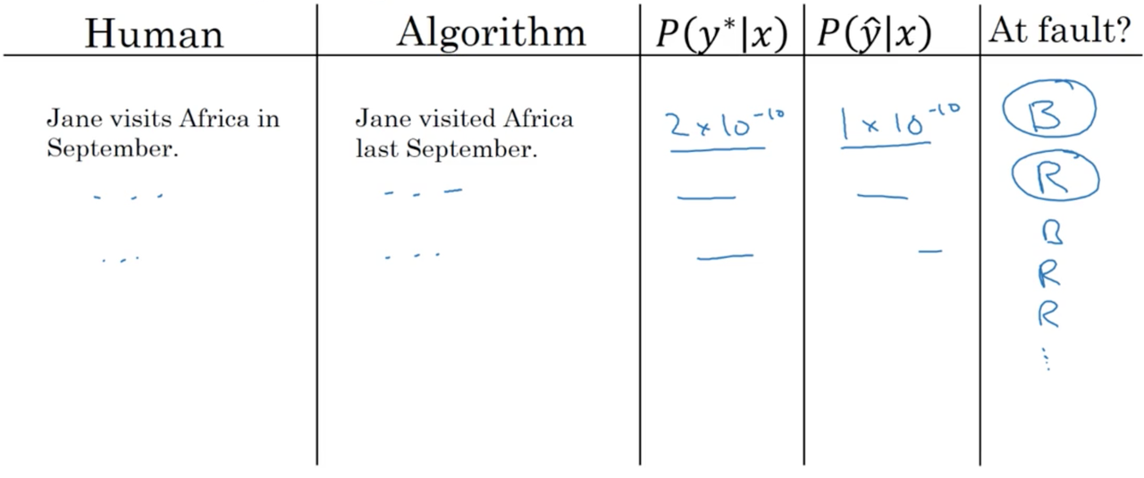
Assume further that our human-provided ($y*)$ and machine provided ($\hat y$) translations for this sentence are:

$$y*: \text{"Jane is visiting Africa in September"}$$

$$\hat y: \text{"Jane visited Africa last September"}$$

Our model has to two main components: our encoder-decoder architecture (which we will simply refer to as our 'RNN' from here on out) and the beam search algorithm applied to the outputs of this RNN. It would be extremely helpful if we could assign blame to one of these components individually when we get a bad translation, like our example $\hat y$.

Similar to how it may be tempting to collect more training data when our models underperform (it 'never hurts'!) it is also tempting in this case to increase the beam width (again, it never seems to hurt!). Error analysis is a more principled way to improve our model, by helping us focus our attention on what is currently hurting performance the most.

Error analysis applied to machine translation

Recall that the RNN computes $P(y | x)$. The first step in our analysis is to compute $P(y* | x)$ and $P(\hat y | x)$. We then ask, which probability is larger? If

Case 1: $P(y* | x)$ > $P(\hat y | x)$

Beam search chose $\hat y$ (recall, its optimization objective is $\hat y = argmax_y P(y|x)$), but $y*$ is more likely according to your model.

Conclusion: We conclude that beam search is at fault. It faild to find a value for $y$ which maximizes $P(y|x)$.

Case 2: $P(y* | x) \le P(\hat y | x)$

$y*$ is a better translation than $\hat y$. But our RNN predicted $P(y* | x) \le P(\hat y | x)$

Conclusion: We conclude that RNN model is at fault. It failed to model a better translation as being more likely than a worse translation for a given input sentence.

Note, we are ignoring length normalization here for simplicity. In reality, you would use the entire optimization objective with length normalization instead of just $P(y|x)$ in your error analysis.

In practice, we might collect some examples of our gold translations (provided by a human) and compare them in a table to the corresponding machine-provided translations, tallying $P(y* | x)$ and $P(\hat y | x)$ for each example. We can then use the rules provided above to assign blame to either the RNN or to beam search in each case:

Through this process, you can carry out error analysis to figure out what fraction of errors are due to beam search versus the RNN model. For every example in your dev sets where the algorithm gives a much worse output than the human translation, you can try to ascribe the error to either the search algorithm or to the objective function, or to the RNN model that generates the objective function that beam search is supposed to be maximizing. If you find that beam search is responsible for a lot of errors, then maybe it is worth increasing the beam width. Whereas in contrast, if you find that the RNN model is at fault, you could do a deeper layer of analysis to try to figure out if you want to add regularization, or get more training data, or try a different network architecture, or something else.

Sequence models & Attention mechanism: Attention Model Intuition

For most of this week, we have been looking at seq2seq models. A simple modification to this architecture makes it much more powerful, lets take a look.

The problem of long sequences

Given a very long French sentence, the encoder in a seq2seq network must read in the whole sentence and then, essentially memorize it by storing its learned representation the activations values. Then the decoder network will then generate the English translation.

$$x: \text{"Jane went to Africa last September and enjoyed the culture and met many wonderful people; she came back raving about how wonderful her trip was, and is tempting me to go too."}$$

Example output (translated sentence)

Now, the way a human translator would translate this sentence is not by reading and memorizing the entire sentence before beginning translation. Instead, the human translator would read the sentence bit-by-bit, translating words as they go, and paying special attention to certain parts of the input sentence when deciding what the ouput sentence should be. For the seq2seq architecture we introduced earlier, we finde that it works quite well for short sentences, but for very long sentences (maybe longer than 30 or 40 words) performance drops.

Short sentences are just hard to translate in general due to the lack of context. For long sentences, the vanilla seq2seq model doesn't do well because it's difficult to for the network to memorize a very long sentence. Blue line: seq2seq architectures without attention, Green line: seq2seq architectures with attention.

In this and the next lecture, you'll see the Attention Model which translates maybe a bit more like humans might, by looking at part of the sentence at a time. With an Attention model, machine translation systems performance stabilizes across sentence lengths. This is mostly due to the fact that, without attention, we are inadvertantly measuring the ability of a neural network to memorize a long sentence which isn't what is most important.

Attention model intuition

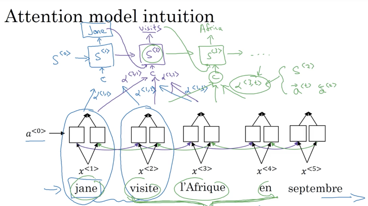
Lets build our intuition for the attention model with a simple example:

$$x: \text{"Jane visite l'Afrique en septembre"}$$

Attention was first introduced here.

Note that attention is typically more useful for longer sequences, but for the purposes of illustration we will use a rather short one.

Say that we use a bi-directional RNN to compute some sort of rich feature set for a given input. Lets introduce a new notation: $\alpha^{<i, j>}$ can be thought of as an attention measure, e.g., when we are looking to produce the translated word $i$ in the output sequence, how much attention should we pay to the word $j$ in the input sequence? Broadly speaking, our decoder takes these measures of attention, along with the output from the encoder network to compute a new input that it uses when determining its outputs. More specifically, $\alpha^{<i, j>}$ is influenced by the forward and backward activations of the encoder network at timestep $i$ and the output from the previous timestep of the decoder network, $S^{<t-1>}$.

Note, we have denoted the activations of the decoder network as $S^{<t>}$ to avoid confusion.

The key intuition is that the decoder network marches away, generating an output at every timestep. The attention weights help the decoder determine what information to pay attention to in the encoders output, as opposed to using all information in the learned representation from the entire input sequence.

Sequence models & Attention mechanism: Attention Model

In the last lecture, we saw how the attention model allows a neural network to pay attention to only part of an input sentence while it's generating a translation, much like a human translator might. Let's now formalize that intuition, and see how we might implement this attention model ourselves.

Attention model

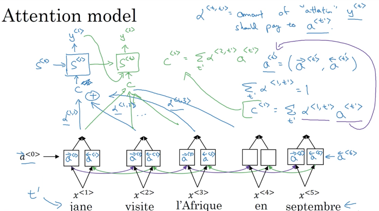
Similar to the last lecture, lets assume we have a bi-directional RNN (be it LSTM or GRU) that we use to compute features for the input sequence.

To simplify the notation, at every timestep we are going to denote the activations for both the forward and backward recurrent networks as $a^{<t>}$, such that:

$$a^{<t'>} = (\overrightarrow{a}^{<t'>}, \overleftarrow{a}^{<t'>})$$

We also have a second RNN (in the forward direction only) with states $S^{<t>}$ which takes as input some context $c$, where $c$ depends on the attention parameters ($\alpha^{<1,1>}, \alpha^{<1,2>}, etc)$. These $\alpha$ parameters tell us how much the context $c$ should depend on the learned features across the timesteps, which is a weighted sum. More formally:

$$\sum_{t'} \alpha^{<1, t'>} = 1$$

$$c^{<1>} = \sum_{t'} \alpha^{<1, t'>}a^{<t'>}$$

In plain english, $\alpha^{<t, t'>}$ is the amount of "attention" that $y^{<t>}$ should pay to $a^{<t'>}$. We compute the context for the second timestep, $c^{<2>}$ in a similar manner:

$$c^{<2>} = \sum_{t'} \alpha^{<2, t'>}a^{<t'>}$$

And so forth and so on.

The only thing left to define is how we actually compute the attention weights, $\alpha^{<t, t'>}$

Computing attentions $\alpha^{<t, t'>}$

Let us first present the formula and then explain it:

$$\alpha^{<t, t'>} = \frac{exp(e^{<t, t'>})}{\sum_{t'=1}^{T_x}exp(e^{<t, t'>})}$$

It is helpful to keep in mind that $\alpha^{<t, t'>}$ is the amount of "attention" that $y^{<t>}$ should pay to $a^{<t'>}$

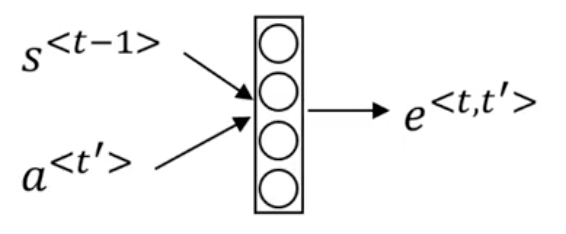
We first compute $e^{<t, t'>}$ and then use what is essentially a softmax over all $t'$ to guarantee that $\alpha^{<t, t'>}$ sums to zero over all $t'$. But how do we compute $e^{<t, t'>}$? Typically we use a small neural network that looks something like the following:

The intuition is, if you want to decide how much attention to pay to the activation of $t'$, we should depend on the hidden state activation from the previous time step, $S^{<t-1>}$ and the learned features of the word at $t'$, $a^{<t'>}$. What we don't know is the exact function which takes in ($S^{<t-1>}, a^{<t'>}$) and maps it to $e^{<t, t'>}$. Therefore, we use a small neural network to learn this function for us.

The network MUST be small as we need to use it to make a prediction at every timestep $t$.

Further reading: Neural machine translation by jointly learning to align and translate and Show, attend and tell: Neural image caption generation with visual attention.

Speech recognition - Audio data: Speech recognition

One of the most exciting developments with sequence-to-sequence models has been the rise of very accurate speech recognition. We will spend the last two lectures building a sense of how these sequence-to-sequence models are applied to audio data, such as the speech.

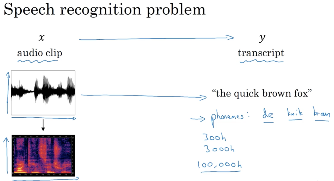
Speech recognition problem

In speech recognition, produce a transcript $y$ given an audio clip, $x$. The audio transcript is generated from a microphone (i.e., someone speaks into a microphone, speech, like all sound, is a pressure wave which the microphone pics up on and generates a spectrum).

In truth, even the human brain doesn't process raw sound. We typically perform a series of pre-processing steps, eventually generating a spectrogram, a 3D representation of sound (x: time, y: frequency, z: amplitude)

The human ear performs something similar to this preprocessing.

Traditionally, speech recognition was solved by first learning to classify phonemes (typically we expensive feature engineering), the individual units of speech. However, with more powerful end-to-end architectures we are finding that explicit phoneme recognition is no longer necessary, or even a good idea. With these arcitectures, a large amount of data is especially important. A large academic dataset may be around 3000h of speech, while commercial systems (e.g. Alex) may be trained on datasets containing as many as 100,000h of speech.

Attention model for speech recognition

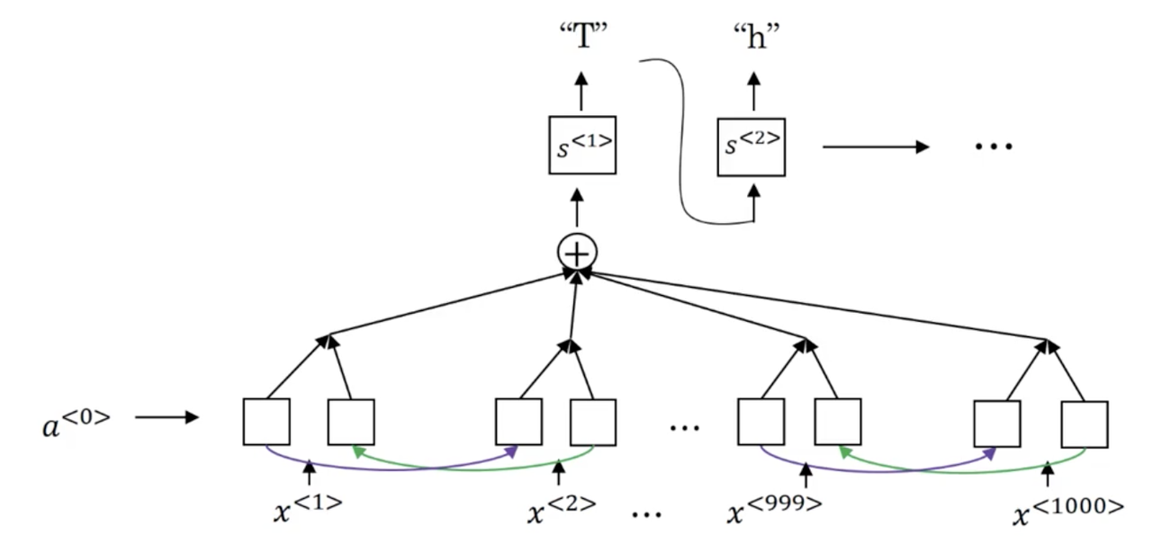
One way to build a speech recognition system is to use the seq2seq model with attention that we explored previously, where the audio clip (divided into small timeframes) is the input and the audio transcript is the output

CTC cost for speech recognition

Lets say our audio clip is someone saying the sentence "the quick brown fox". Typically in speech recognition, the length of our input sequence is much much larger than the length of our output sequence.

For example, a 10 second, 100 Hz audio clip becomes a 1000 inputs.

Connectionist temporal classification (CTC) allows us use a bi-directional RNN where $T_x == T_y$, by allowing the model to predict both repeated characters and "blanks". For our examples, the predicted transcript might look like:

$$\text{ttt _ h _ eee _ _ _ _ <SPACE> _ _ _ qqq _ _ ...}$$

Where _ denotes a "blank".

The basic rule is to collapse repeated characters not separated by a "blank".

This idea was originally introduced here

Summary

In this lecture we tried to get a rough sense of how speech recognition models work. We saw:

• two methods for building a speech recognition system (both involved bi-directional RNNs): a seq2seq model with attention and a CTC model.
• that deep learning has had a dramatic impact of the viability of commercial speech recognition systems.
• building effective speech recognition system is still requires a very significant effort and a very large data set.

Speech recognition - Audio data: Trigger word detection

Trigger word detection systems are used to identify wake (or trigger) words (e.g. "Hey Google", "Alexa"), typically for digital assistants like Alexa, Google Home and Siri.

The literature on trigger word detection is still evolving, and there is not widespread consensus or a universally agreed upon algorithm for trigger detection. We are just going to look at one example.

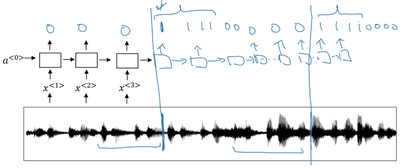
Our task is to take an audio clip, possibly perform preprocessing to compute a spectrogram and then the features that we will eventually pass to an RNN, and predict at which timesteps the wake word was uttered. One strategy, is to have the neural network output the label 0 for all timesteps before a wake word is mentioned and then 1 directly after it is mentioned. The slight problem with this is that our training set becomes very unbalanced (many more 0's than 1's). Instead, we typically have the model predict a few 1's for the timesteps that come directly after the wake word was mentioned.